Getting the most benefit out DB2 for i requires keeping the concept of "set at time" in mind and making use of all the latest features and functions.
By Mike Cain
In Dan Cruikshank's August 2008 article "Working with Data Sets," Dan illuminated the power of SQL "set at a time" processing, and he used some of the new DB2 for i 6.1 OLAP functions to do it. In this article, I'll expand on this concept and demonstrate some additional uses for OLAP functions, as well as reiterate the reasons that SQL can be so powerful for the data-centric programmer. We'll also take a look at some of the performance considerations for more-complex SQL requests.
First, a review of the SQL OLAP functions available as described in the DB2 for i SQL Reference publication:
•· RANK or DENSE_RANK specifies that the ordinal rank of a row within the window is computed. Rows that are not distinct with respect to the ordering within their window are assigned the same rank. The results of ranking may be defined with or without gaps in the numbers resulting from duplicate values.
RANK specifies that the rank of a row is defined as 1 plus the number of rows that strictly precede the row. Thus, if two or more rows are not distinct with respect to the ordering, there will be one or more gaps in the sequential rank numbering.
DENSE_RANK specifies that the rank of a row is defined as 1 plus the number of preceding rows that are distinct with respect to the ordering. Therefore, there will be no gaps in the sequential rank numbering.
•· ROW_NUMBER specifies that a sequential row number is computed for the row within the window defined by the ordering, starting with 1 for the first row. If the ORDER BY clause is not specified in the window, the row numbers are assigned to the rows in arbitrary order, as returned by the subselect (not according to any ORDER BY clause in the SELECT statement).
•· GROUPING SETS allows multiple grouping clauses to be specified in a single statement. This can be thought of as the union of two or more groups of rows into a single result set.
•· ROLLUP is an extension to the GROUP BY clause that produces a result set containing subtotal rows in addition to the ″regular″ grouped rows. Subtotal rows are ″super aggregate″ rows that contain further aggregates whose values are derived by applying the same column functions that were used to obtain the grouped rows.
•· CUBE is an extension to the GROUP BY clause that produces a result set that contains all the rows of a ROLLUP aggregation and, in addition, contains ″cross-tabulation″ rows. Cross-tabulation rows are additional ″super aggregate″ rows that are not part of an aggregation with subtotals.
To set up our simple example, let's assume we have three tables that describe students, classes enrolled in, and activities signed up for (Figure 1). The classes and activities are related to students by the studentid column.
create table students (studentid int, studentname char(20));
create table classes (studentid int, class char(20), fee decimal(7,2));
create table activities (studentid int, activity char(20), fee decimal(7,2));
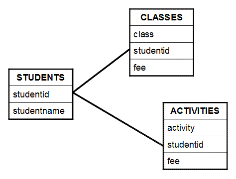
Figure 1: Our example shows students and their classes and activities.
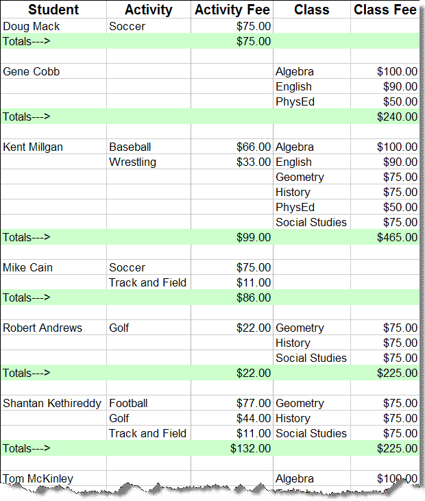
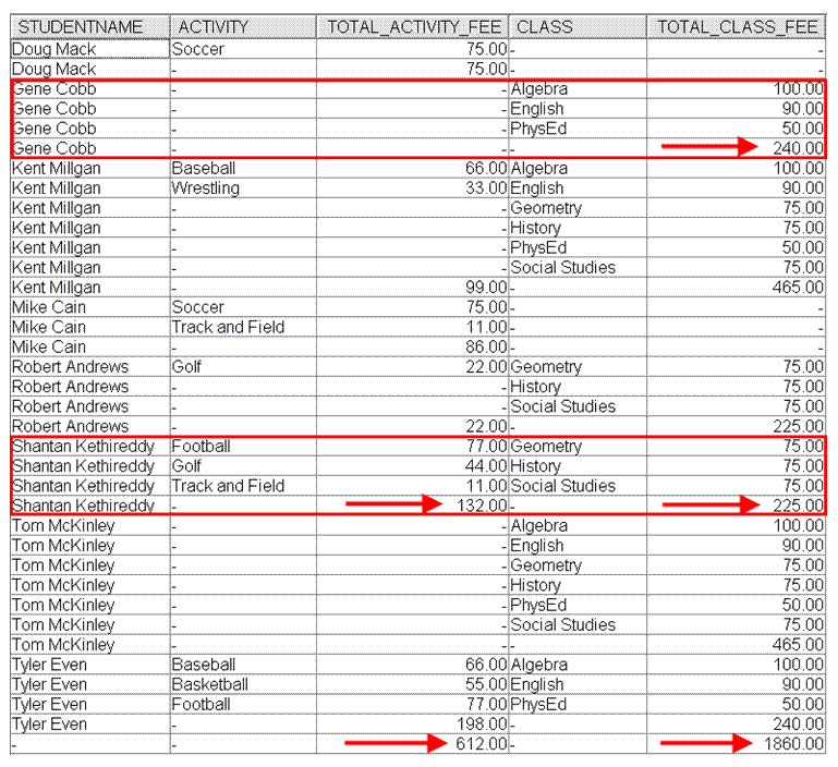
Our job is to produce a report that shows all students along with their respective classes and activities, the fees associated with each class and activity, the total class and activity fees for each student, and a final total of all fees represented in the set (Figure 2).
Figure 2: All students' class and activity costs are totaled. (Click images to enlarge.)
Looking at the report, we see that the various activities and classes for each student are not related, yet we need to fully populate each line of the report with information. At first blush, this is not a trivial task, especially if we want to minimize the number of passes through the data. Enter SQL and OLAP functions.
To understand how to accomplish this with SQL, we must recognize the work that needs to be done based on the given data model.
For each student, we must list the classes and the fees associated with these classes, calculate the total fees, and then order by student. The following SQL statement represents this request:
select s.studentname,
c.class,
sum(fee) as total_class_fee
from students s,
classes c
where s.studentid = c.studentid
group by s.studentname,
c.class
order by s.studentname;
For each student, we must also list the activities and the fees associated with these activities, calculate the total fees, and then order by student. The following SQL statement represents this request:
select s.studentname,
a.activity,
sum(fee) as total_activity_fee
from students s,
activities a
where s.studentid = a.studentid
group by s.studentname,
a.activity
order by s.studentname;
If we were to union the two results together, we would most certainly provide all the results in one set, but the report will contains holes or gaps. In other words, the rows representing classes and activities for each student will be listed vertically, not horizontally. We need to somehow get the class and activity information condensed into as few rows as possible. We need to "drill across" each set of results to find all classes and activities for each student (Figure 3). In effect, we are pivoting either the class information or the activity information up so that it appears alongside the student information horizontally.
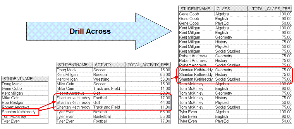
Figure 3: Drill across the result sets.
The big question is, how do we accomplish this with SQL against our simple relational data model? Part of the answer entails using a left outer join. Specifically, using the distinct set of students on the left and joining to their respective class and activity information on the right. By using a left outer join, the database engine will return the student information even if there is no corresponding class or activity for that student.
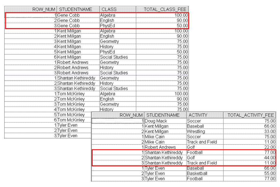
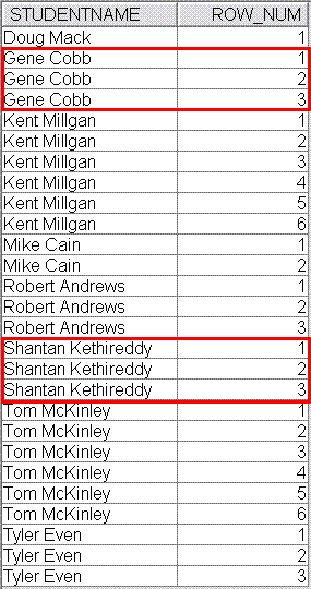
But how do we know if a student is associated with any activities or classes? And how do we determine the number of lines each student will need to represent their condensed list of classes and activities? Enter ROW_NUMBER OVER. With the ROW_NUMBER function, we can have DB2 assign a number to each intermediate result and use it later. Furthermore, if we use the OVER clause, PARTITION BY clause, and ORDER BY clause, we are able to assign distinct numbers to each result, by student, and have these results ordered by class or activity (Figure 4). We will include grouping criteria in case the student is signed up for the same class or activity more than once. The enhanced SQL statements would like this:
select ROW_NUMBER() OVER (PARTITION BY s.studentname
ORDER BY c.class) AS row_num,
s.studentname,
c.class,
sum(fee) as total_class_fee
from students s,
classes c
where s.studentid = c.studentid
group by s.studentname,
c.class
order by s.studentname,
row_num;
select ROW_NUMBER() OVER (PARTITION BY s.studentname
ORDER BY a.activity) AS row_num,
s.studentname,
a.activity,
sum(fee) as total_activity_fee
from students s,
activities a
where s.studentid = a.studentid
group by s.studentname,
a.activity
order by s.studentname,
row_num;
Figure 4: The results are ordered and numbered.
Notice that each student now has his respective classes and/or activities ordered and numbered. Keep in mind that the row number is actually part of the result set.
To obtain the list of students who have classes, activities, or both, we can run the following statement against the results from classes and activities. Recall that UNION removes duplicates for the result set. Also notice that we want to order the results by studentname and the row number assigned by DB2 (Figure 5).
select studentname,
row_num
from intermediate results from the previous query - Figure 4
union
select studentname,
row_num
from intermediate results from the previous query - Figure 4
order by studentname,
row_num;
Figure 5: These are the results of merging the lists together via UNION.
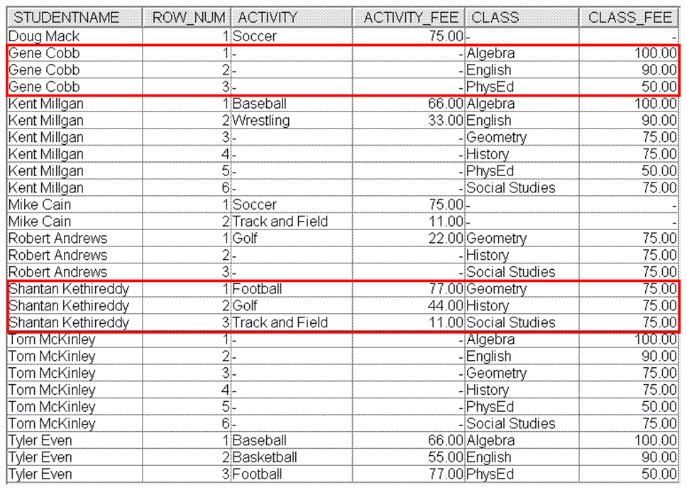
The result set tells us not only the students who have either classes or activities, but also how many lines it will take to show the information. As the next step in the process, this list of distinct studentnames and row numbers will be used to drill across the classes and activities via a left outer join.
select t3.studentname,
t3.row_num,
t1.activity,
sum(t1.total_activity_fee),
t2.class,
sum(t2.total_class_fee)
from intermediate results from the previous query - Figure 5
left outer join intermediate results from the previous query - Figure 4
on (t3.studentname = t1.studentname
and t3.row_num = t1.row_num)
left outer join intermediate results from the previous query - Figure 4
on (t3.studentname = t2.studentname
and t3.row_num = t2.row_num)
order by t3.studentname,
t3.row_num
t1.activity,
t2.class;
The results of the left outer joins might look like this (Figure 6):
Figure 6: Here are the results of a left outer join.
Now that we have each student's information condensed into the fewest number of lines required, we can turn our attention to providing class and activity fee totals by student and ordering the results (Figure 7). For this, we will use the new OLAP feature grouping sets. In our report, we have three sets of grouping criteria to sum up: fees for each line of the report, fees for each student, and grand totals for the report--namely (studentname, row_num, activity, class), (studentname), and (). The SQL used to drill across and aggregate the data looks like this:
select t3.studentname,
t1.activity,
sum(t1.total_activity_fee),
t2.class,
sum(t2.total_class_fee)
from intermediate results from the previous query - Figure 5
left outer join intermediate results from the previous query - Figure 4
on (t3.studentname = t1.studentname
and t3.row_num = t1.row_num)
left outer join intermediate results from the previous query - Figure 4
on (t3.studentname = t2.studentname
and t3.row_num = t2.row_num)
group by grouping sets ((t3.studentname, t1.activity, t2.class),
(t3.studentname),
())
order by t3.studentname,
t1.activity,
t2.class;
Figure 7: Now, we have class and activity fee totals by student.
Now that we have the various pieces and parts to arrive at our final data set, let's put it all together. While we certainly could use multiple SQL statements and actual intermediate tables to do this, let's use the power of DB2 to do all of this work with one SQL statement. To do this, we will take advantage of common table expressions. Recall that a common table expression permits us to define a result table (with a table identifier) that can be specified as a table name in any FROM clause of the full select that follows. This will allow us to define and build all of our various intermediate results and then perform the left outer join and grouping--in one SQL request. Doing this also has the advantage of allowing the DB2 for i optimizer and database engine to perform all the work in microcode, eliminating the need to materialize true temporary tables. It is also possible that there will be additional benefit from overlapping I/O and data reuse. We should also add the OPTIMIZE FOR ALL ROWS clause because our application will fetch and consume all of the query results without waiting. Here is the single SQL statement to do all the work I have described previously:
with t1 as
(
select ROW_NUMBER() OVER (PARTITION BY s.studentname ORDER BY a.activity) AS row_num,
s.studentname,
a.activity,
sum(fee) as total_activity_fee
from students s, activities a
where s.studentid = a.studentid
group by s.studentname, a.activity
),
t2 as
(
select ROW_NUMBER() OVER (PARTITION BY s.studentname ORDER BY c.class) AS row_num,
s.studentname,
c.class,
sum(fee) as total_class_fee
from students s, classes c
where s.studentid = c.studentid
group by s.studentname, c.class
),
t3 as
(
select studentname, row_num
from t1
union
select studentname, row_num
from t2
)
select t3.studentname, t1.activity, sum(t1.total_activity_fee) as Total_Activity_Fee, t2.class,
sum(t2.total_class_fee) as Total_Class_Fee
from t3
left outer join t1 on (t3.studentname = t1.studentname AND t3.row_num = t1.row_num)
left outer join t2 on (t3.studentname = t2.studentname AND t3.row_num = t2.row_num)
group by grouping sets (
(t3.studentname, t3.row_num, t1.activity, t2.class),
(t3.studentname),
()
)
order by t3.studentname, t1.activity, t2.class
optimize for all rows;
Now that we have our SQL statement built and tested, let's turn our attention to performance. Using the advanced System i Navigator tools such as Visual Explain, we can see the "out of the box" plan for this query (Figure 8). We can also make use of the index advice provided automatically by DB2 for i.
Figure 8: This is the plan for our query.
Focusing on the top, rightmost nodes, we can see that the plan involves full scans on the tables: students, activities, and classes (Figure 9). This makes sense, given there are no local selection predicates for any of the tables. The inner join order is students, then activities and students, and then classes. To accomplish the joins, hash tables are built and probed. This makes sense, given there are no indexes available to facilitate joins by key.
Figure 9: We accomplish the joins by using hash tables.
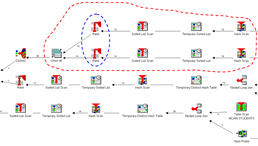
The results of the inner joins are sorted and placed in temporary lists. These sorted lists will be used to support the row-number processing. This is represented by the ranking nodes. The intermediate results are then combined via the UNION (Figure 10).
Figure 10: The intermediate results are combined via the UNION.
The results of the UNION operation are then left outer joined on studentname and row_num to the earlier intermediate results (Figure 11). These results are sorted and placed in a temporary list with duplicates removed.
Figure 11: The UNION results are left outer joined on studentname and row_num.
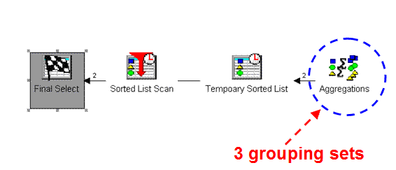
The final, single, sorted list will be used to support the three levels of aggregations specified by the grouping sets. All three totals are calculated with one pass of the data coming from the previous join results (Figure 12). The aggregated results are sorted based on the order by criteria and delivered to the user.
Figure 12: The totals are calculated.
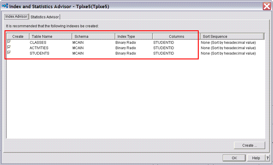
To tune up our query, we can take advantage of the DB2 for i index advisor. The indexes being advised can be found in the table QSYS2.SYSIXADV by using the Navigator. In our case, we are invoking the advisor from Visual Explain and can see that three indexes are being suggested:
Figure 13: The index advisor suggests three indexes.
To support the joins between students and their classes and activities, we would provide indexes on the respective join columns, such as this:
create index students_ix1 on students (studentid);
create index activities_ix1 on activities (studentid);
create index classes_ix1 on classes (studentid);
These indexes will give the DB2 for i query optimizer more information about the data and provide another option for joining the tables--namely, nested loop join by key. Ultimately, the optimizer will choose what it calculated as the fastest plan for your query, against your data, on your system.
If for our report we wanted to select only one student, by name, we would modify the query to have a local selection predicate. We should also provide additional indexes to support the local selection-plus-join conditions. Our new SQL request might look like this:
with t1 as
(
select ROW_NUMBER() OVER (PARTITION BY s.studentname ORDER BY a.activity) AS row_num,
s.studentname,
a.activity,
sum(fee) as total_activity_fee
from students s, activities a
where s.studentid = a.studentid
group by s.studentname, a.activity
),
t2 as
(
select ROW_NUMBER() OVER (PARTITION BY s.studentname ORDER BY c.class) AS row_num,
s.studentname,
c.class,
sum(fee) as total_class_fee
from students s, classes c
where s.studentid = c.studentid
group by s.studentname, c.class
),
t3 as
(
select studentname, row_num
from t1
union
select studentname, row_num
from t2
)
select t3.studentname, t1.activity, sum(t1.total_activity_fee) as Total_Activity_Fee, t2.class,
sum(t2.total_class_fee) as Total_Class_Fee
from t3
left outer join t1 on (t3.studentname = t1.studentname AND t3.row_num = t1.row_num)
left outer join t2 on (t3.studentname = t2.studentname AND t3.row_num = t2.row_num)
where t3.studentname = 'Mike Cain'
group by grouping sets (
(t3.studentname, t3.row_num, t1.activity, t2.class),
(t3.studentname),
()
)
order by t3.studentname, t1.activity, t2.class
optimize for all rows;
And to avoid full table scans, our supporting indexes would be these:
create index students_ix2 on students (studentname, studentid);
create index activities_ix2 on activities (studentname, studentid);
create index classes_ix2 on classes (studentname, studentid);
For this scenario, it would be perfectly acceptable to have all six indexes in place. These indexes will be available to handle the request for all students, as well as a particular set of students, as specified in the WHERE clause.
Furthermore, if this report would be expected to query, process, and return a much larger set of rows, then the optional DB2 Symmetric Multiprocessing feature could be employed to provide parallel processing. This might entail parallel table scans to read the base tables and populate the hash tables, as well as run the joins in parallel. If multiple CPUs and a supporting I/O subsystem were in place, SMP could possibly provide a significant performance increase and lower the response time.
As you can see, SQL is a very powerful and robust language. Getting the most benefit out DB2 for i requires keeping the concept of "set at time" in mind and making use of all the latest features and functions. You can use this drill-across technique to handle situations where you need to place related or unrelated figures next to each other horizontally, such as drilling across and combining measures from two or more fact tables by subject.
For more information and details regarding the DB2 for i OLAP functions, be sure to review the 6.1 DB2 for i SQL Reference.






 Business users want new applications now. Market and regulatory pressures require faster application updates and delivery into production. Your IBM i developers may be approaching retirement, and you see no sure way to fill their positions with experienced developers. In addition, you may be caught between maintaining your existing applications and the uncertainty of moving to something new.
 IT managers hoping to find new IBM i talent are discovering that the pool of experienced RPG programmers and operators or administrators with intimate knowledge of the operating system and the applications that run on it is small. This begs the question: How will you manage the platform that supports such a big part of your business? This guide offers strategies and software suggestions to help you plan IT staffing and resources and smooth the transition after your AS/400 talent retires. Read on to learn:
LATEST COMMENTS
MC Press Online